
To come to the point: We are not friends of the risk matrix (heat map), but we have to admit that it is still used in many areas.
As the aim of the layout of a typewriter keyboard was to break the flow of writing as little as possible, the task of the risk matrix (heat map) is to simplify the representation of threats. It must be taken into account that in the early days of the risk matrix, quantitative more convincing instruments such as the Monte Carlo approach required a lot of time to use it as a decision-relevant instrument. According to economists, the continued widespread use of the risk matrix is due to path dependencies: People are familiar with depicting risks using a matrix.
For those decision driven people, which still have to use "heat maps" to communicate threats, MC FLO offers an equivalent instrument - the conditional risk matrix. Let's start....
The "raison d'être" of a comprehensive quantitative analysis using the Monte Carlo approach is an objectively justifiable recommendation for a decision, taking into account uncertainty.
In the context of classic corporate planning, the primary goal is to generate an economic profit, which for most corporate companies can be derived approximately using the sum of the cash flows from operations (including the interest burden for borrowed capital) and investment activities. The minimum target is an economic profit of 0; this ensures that all claimants from suppliers, employees and lenders can be met to the extent that there is still enough space for necessary investments in tangible and intangible assets. The purpose of corporate planning is thus to identify the relevant drivers to achieve the primary goal.
From our point of view, only a quantitative analysis is able to do this, since the management is very often confronted with the same questions: “What will happen if sales volume collapses by x%? How confident can we be that the profit is positive?". We advocate an approach in which «knowledge» (beliefs) and data flows into the decision-making process (Bayesian inference). In this way, the qualitative analysis can be converted into a quantitative one. The target value is thus described as a range using a probability estimate ("what is the probability [or also the degree of belief] that the free cash flow in the planning period will be at least CHF 0?").
Let's take a closer look at the basic example supplied with MC FLO ("MC FLO Test.xlsx")*. In addition to the sales volumes for the product, assumptions must be made about prices, growth, costs and a "jump factor".
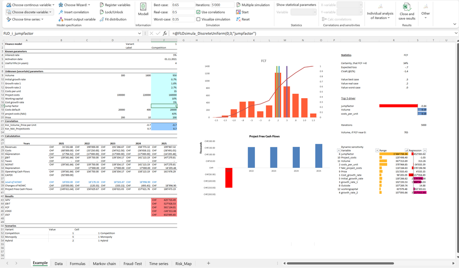
The traditional planning process often separates the drivers: costs and sales volume are quantified and transferred to the planning tool; rather a-priori qualitative artifacts such as potential "jump factors" at best as a scenario, at worst as part of a separate risk analysis using a risk heat map and thus withdrawn from an integrated quantitative analysis. Things get worst, if the relevant drivers are incorporated as part of the corporate plan and into a separated risk analysis.
However, MC FLO allows to deviate automatically the risk heat map from the corporate plan, as shown below (we assume, that our goal is to earn a FCF of at least 0 CHF and the ambition on all variables is set at P65).
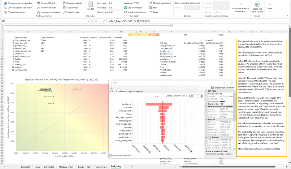
We have derived the values of the risk matrix in columns O and P - parting from the target value defined in cells I1: K1. The probability that the FCF falls below CHF 0, given that the variable "Volume" does not exceed the value at P65 of 1'142 units (cell H13; ie: P65 i.e. 65% of the results to the quantities are below the threshold of 1,142**), is approx. 39% (cell O15)***. The average damage if the FCF falls below CHF 0, given that the variable "Volume" is lower than 1,142 units, is roughly MCHF 0.49 (cell P15). Combinations in which the conditional probability and the conditional severity are high, for example in the case of the variable “jumpfactor”, are therefore dangerous. Accordingly, the variable "jumpfactor" is shown in the conditional risk matrix in the red area. The equivalent in the dynamic sensitivity analysis is the classification of the variable “jumpfactor” at the top of the corresponding diagram. It can be seen that a change in the "jumpfactor" has a clear influence on the average expected value of the FCF. The next entry in the dynamic sensitivity analysis is the “Volume” variable, followed by the “costs_per_unit” variable. Overall, however, the effect for the costs_per_unit variable is small, which leads to a classification in the yellow area of the risk matrix.
From a management perspective, a red classification means that the corresponding variables have a high influence on our targets and must therefore be managed first. In our case, this applies only to the variable “jumpfactor”.
Although the automated conditional risk matrix is mostly consistent with the dynamic sensitivity analysis, there are some potential drawbacks. Let's adjust the model so that the costs per unit can vary between CHF 3,000 and CHF 4,000 and thus the probability of generating an FCF of less than CHF 0 is 100% (the probability of lifting the FCF above CHF 0 is therefore 0%).
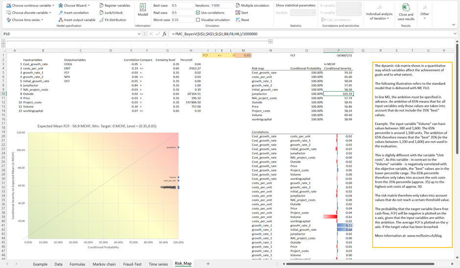
In this case, all variables are on the right vertical line of the conditional risk matrix, and here too the variable “jumpfactor” is identified as the most influential driver. With this model constellation, however, there is no option to sustain the company.
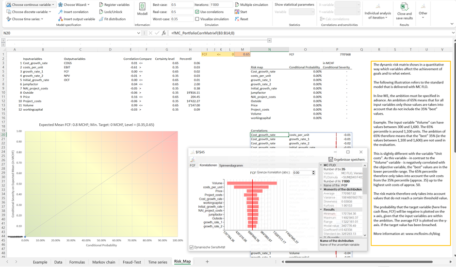
The case looks a little different if the probability of earning an FCF less than CHF 0 is 0%. For this purpose, we allow the unit costs to vary between CHF 0.3 and CHF 0.4 compared to the original model and limit the maximum value of the project costs to CHF 22,000. Now all variables in the conditional risk matrix are on the bottom left. Given that an adjustment of the individual variables does not lead to an FCF less than CHF 0, the corresponding probabilities are also 0%, which explains the concentration on one point (in the green area). You can lay down and let chance rule. In no case - given the model specification - a FCF of less than CHF 0 is expected.
The dynamic sensitivity analysis, on the other hand, shows which variables have the greatest influence on the FCF, regardless of the objectives to be met.
The conditional risk matrix spans the result of a dynamic sensitivity analysis into the dimensions "(conditional)probability of occurrence" and "conditional severity"; however, it is not possible to multiply these variables to combine them, since the base is different in each case. The assessment of the probability of occurrence is based on the following question: “How likely is it that the FCF is less than 0, given that the variable "Volume" is less than 1,142?”. In the case of the dimension "conditional severity" the question is as follows: "How high will the loss of the FCF be, given that the variable "Volume" is less than 1,141 and the FCF is less than 0?". The condition is therefore linked to the "Volume" variable and a previously defined FCF level.
One last point: Although the x-axis is limited between 0% and 100%, there is no limit for the y-axis. Here it is important to define a limit in advance of the maximum loss that can be borne (or insured). In contrary you may be trapped by the illusion that a "yellow" or "green" rating does not pose threats.
Prologue: A disadvantage of the risk matrix is that it does not underline dependencies between the individual variables. With the function fmc_PortfolioCorrMatrixF built into MC FLO, all correlations with the respective correlation coefficients (Pearson or Spearman) can be made visible.
Conclusion: The conditional risk matrix, using the dimensions "conditional probability" and "conditional severity" is a valid Instrument to manage goals in an efficient way, preserving the known visual representation of threats using a risk heat map.
*The standard example only consists of a simplified cash flow calculation; An example of an integrated corporate planning approach using Monte-Carlo simulation and the ability to update the assumed beliefs with given new data (Bayesian inference) can be requested by sending an email to support@mcflosim.ch (you need a perpetual license).
**Whether P65 or (1-P65) is used depends on the sign of the correlation coefficient with the goal variable - here FCF. The variable "Volume" (amount) is positively correlated with the FCF. The P65 level "eliminates" the 35% highest quantities from the "Volume" distribution (this corresponds to the right edge of the distribution function). The unit costs, on the other hand, are negatively correlated with the FCF. In this case, the P65 level eliminates the 35% lowest unit costs from the "cost_per_unit" distribution (this corresponds to the left edge of the distribution function). The choice of the Px value - also known as the ambition level - is company specific. Of course, a different level of ambition can be defined for each variable. An analogous interpretation can be made using the "value-at-risk" approach.
***All other input variables are used in a consistent way - taking into account dependencies.
Kommentar schreiben