Time series - some notes with regard to the geometric Brownian motion

From some customers we received questions about the correct handling of MC FLO in the context of time series. In the present article we will deepen the typical questions with a simple example concerning the geometric Brownian motion.

With MC FLO we have created a product that is very easy to use, and we are convinced that it should remain so in the future. Therefore, we consciously avoid formulas or constructs that cause many headaches in daily use with Excel. It strikes out, that the array formula is such an example. Disadvantages of array functions are the cumbersome handling and the lack of transparency about the determination of the individual elements of an array. With the omission of array functions in MC FLO, therefore, other ways must be taken.

Let's us look at the following example:
You have the task to plan the product sales for the next five periods. Both the price and the quantity are considered uncertain. For the quantity you assume a lognormal distribution. For the price, you want to assume a geometric Brownian motion with starting value 100 (all parameters can be taken from the enclosed Excel). Excel professionals would now expect that the price path is modeled using an array function in lines E7: I7. Not so with MC FLO.

With MC FLO you have several options to bypass the array function and still map a robust derivation of the geometric Brownian motion series with few simple steps in Excel, at least as an approximation.

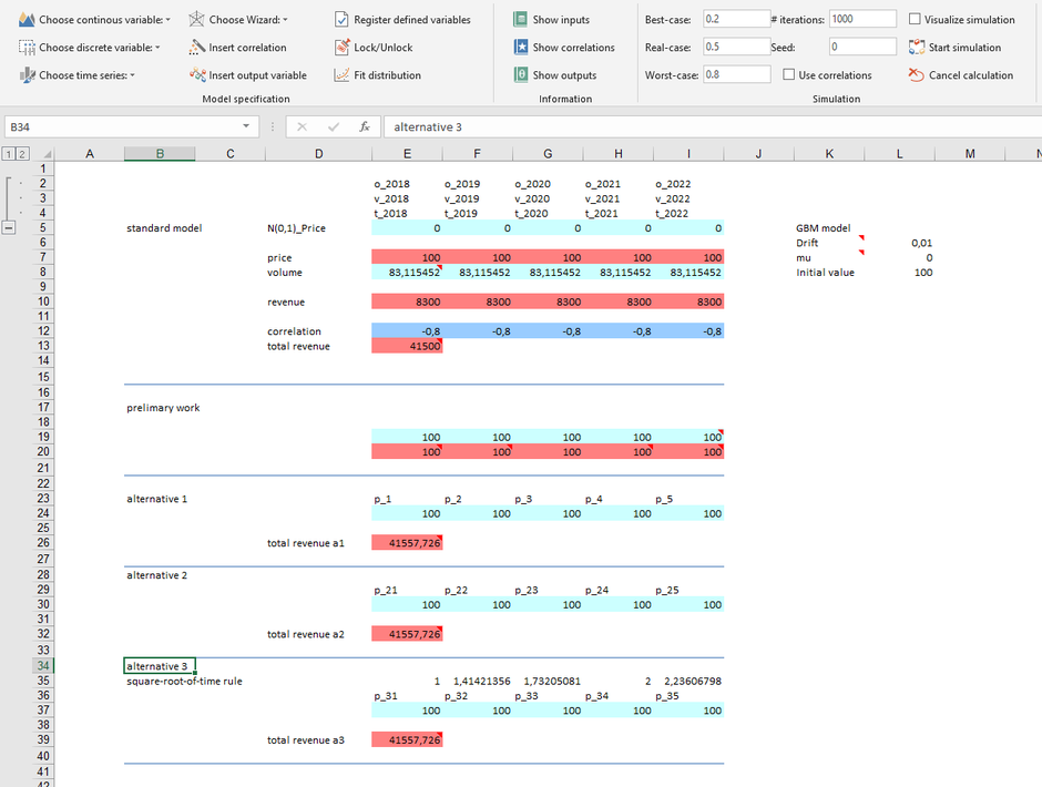
The first strategy is to enter a separate time series formula for each time period, which we did in lines E24: I24 (alternative 1). As a special feature we have used the previous cell as the start value and set the flag to "1" for the parameter "UseBefore". This ensures that the calculated value of the predecessor (eg line E24) is used as the start value for the next period (cell F24). What sounds obvious at first sight, however, requires clarification. The formulas given in cells E24: I24 change with each iteration. For example, if you want to perform a simulation with 5,000 iterations, in our case this means that the formula entered in cell E24 can take a value between 8 and 1,250 monetary units, reflecting the volatility within 5'000 time periods (see cell H20).

The logic is very simple: A simulation with 5,000 iterations of a time series variable is comparable to the determination of a time series over 5,000 periods! In five consecutive periods, however, such a large deviation cannot be expected with the parameters defined. If you want to explicitly work with time series in this case, there are two ways out: the first is to adjust the formula for each variable (for example, by massively reducing the drift parameter). Thus, you can model a more realistic path of the price development over the five periods even with several thousand iterations. How do we come up with the new parameters? In cell E20 we have shown the result of the time series with the output parameters of the geometric Brownian motion series over the five periods after 5,000 iterations. The values vary between 92 and 107 price units.

In cell I20 we have entered new parameters for a geometric Brownian series by trial and error, which at 5,000 iterations approximate the values of 92 and 107 mentioned above. The result can be taken from the cell I21. In cells E21: I21, this new formula has been entered. The result of the geometrically Brownian series adapted to the number of iterations can be found in cell E26.

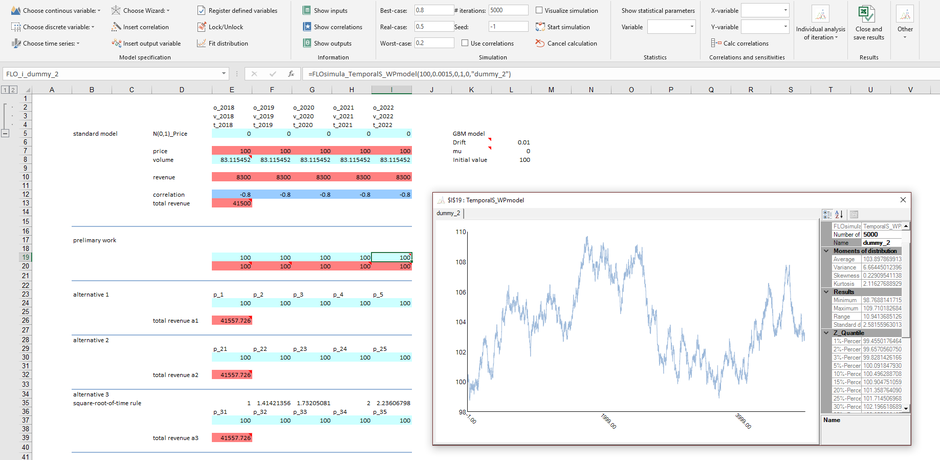
The second option is to specify the number of periods in the original formula as an additional parameter and leave the starting value at 100 (alternative 2). We have reintroduced this alternative in lines E30: I30. So, for the second period, the formula is "= FLOsimula_TemporalS_WPmodel (100; 0.01; 0; 1; 0;" p_22 "; 2)", where 2 before the closing bracket defines the number of periods. For each of the 5,000 iteration runs, the value for the second period (per end) is calculated starting from the initial value of 100. In cell I30, the same logic occurs for the fifth period.

Both possibilities using explicitly time series function have major drawbacks: we must first perform a transformation (in the first case) or we are not able to take into full account correlations (in the second case).

But we have two other options.

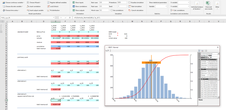
The third possibility is to map the possible characteristics in each planning period using a density or distribution function. The geometric Brownian motion series follows in term of prices a log-normal distribution (prices are never less than 0), while the returns (the deviations between two periods) are normally distributed. If we interpret the price evolution over the five periods as the result of a return distribution, we can approximate the behavior of the price path with a normal distribution, whereby the standard deviation increases over time based on the square root of time rule. This alternative is shown in lines E37: I37. In doing so, we obtained the parameters of the normal distribution using the same logic (trial-and-error) as with alternative 1. In line G19 we have shown the possible occurrences of the time series over the period. The result can then also be taken from G20. The values thus fluctuate between 96 and 104 in cell E37.

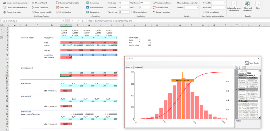
The last solution, favored by us, is to derive the price development directly using the formula for the geometric Brownian motion in Excel, which we did in cells E7: I7 and using output variables of MC FLO. The starting point is a standard normal distribution which, parting with cell E5, is assembled to the desired price path.

For all alternatives as well as for the standard solution, we registered the formulas automatically in Excel and MC FLO using the function "Register defined variables" (see also the following video). This ensures that the modelling takes place as quickly as using an array function. The advantage compared to the array function is that all variables, even the random terms of a time series, are made transparent and hence a detailed tracking of the result is guaranteed.

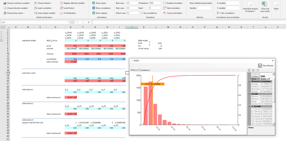
We will assume a negative correlation of -0.8 between prices and volume sales. Since we have identified the random terms of the time series in the preferred solution, we can map a corresponding correlation between the volume and the random term of the geometrically Brownian motion without further effort. So easy. With MC FLO you will then be able to identify rapidly which variables significantly influence the total sales over all five periods, which we have outlined by the the tornado diagram of MC FLO. If you look at the correlation between the amount in 2018 ("v_2018") and the price for 2018 ("p_2018") in the result workbook, you will notice that the correlation is not -0.8, which can partly be explained by the fact that the price is composed only partly by the random component which prevents a correlation of exactly -0.8 in any case.

In the blog for the AR (1), MA (1) - both in German - and here for the geometrically Brownian motion (GBM) we have shown the necessary steps how to use time series in MC FLO without the use of an array function. With the time series built into MC FLO, you can simulate several thousand periods for individual variables, or even more importantly, they support forecasts. With future blog contributions to the ARMA (1,1) and ARCH(1) process we'll continue our journey with the time series implemented in MC FLO.