
In MC FLO you have three alternative to make a Monte Carlo simulation. The first can be called the classic mode. Here, you define the input variables graphically and specify the output variables linking the desired cells in the Excel workbook. After the simulation, you receive the results in a separate Excel workbook, which you can integrate into any other workbook or make it available to others. With the second mode - the preview mode - you can preview the simulation results of all input variables and correlations according to the specification of the model and, by clicking on the corresponding output variable, you can also preview the simulation results of the output variables. With "Copy + Paste" you have no limits to copy the results (such as the percentiles) without having to start the classic simulation run. For time series, however, this step can be tedious, since a process must first be defined for the historical data, and only then a calculation can be triggered. For a well-founded prognosis, which should be executed without any identification of other statistical key figures, we offer starting from version Santiago III also a batch function, which carries out the steps described above automatically.
Assume that you as a hotel manager have collected the occupancy of your hotels for the months March 2017 - March 2018 on a weekly basis and you want to make an occupancy forecast for the next seven weeks, using the last week as the basis for ordering the goods and scheduling (the Excel can be found here, all labels are in german instead).
Starting with Excel 2016, you can use the "forecasting tool" function, which uses triple exponential smoothing as an example of a deterministic procedure (in the example below, we have introduced the function "= FORECAST.ETS (DU3; $ E$4:$DZ$4;$E$3:$DZ$3)», starting with line DU20). In many cases, exponential smoothing as an ad hoc prognosis is perfectly adequate. However, if you want to examine the internal structure of the data in more detail, gain insights into the logic of the process, and easily create a risk-based forecast, we recommend that you analyze the data using a time series process as implemented in MC FLO.
A time series is captured as an object of two parts: a basic component (such as the mean) and an invisible random component that overlays the fundamental component. Sometimes these random components correlate over time (which establishes a moving average process [MA]) or the observed data points correlate directly with each other (which corresponds to an auto-regressive process [AR]). A combination of both defines the ARMA process. In AR, MA or in general the ARMA processes, it is necessary that they have no trend or seasonal effects. If this is the case, the time series should be transferred to a stationary time series (see also our blog, in german), which we ignore here. In the development of MC FLO we are guided by daily practice and this undoubtly means that the path of least resistance has to be taken. So it is often the case that a prognosis is made periodically for a fixed number of data points and that the forecast should be automated. In our case, a new prognosis for the following seven weeks should be carried out next week. Since forecasts in the context of a simulation should always be understood as a concept of bandwidth planning, an ad-hoc forecast should be used as flexibly as possible and using risk-related statements ("probability") for confidence leves. Heard, done. In our hotel example, we've added the new function implemented with Santiago III: "= fMC_Batch_Time ($E$4:$ZZ$4;7;1;0;10000;0.95)" with the appropriate parameters in line 25. This has the task to create a prognosis for the next seven periods from the existing actual numbers of lines E to ZZ. A time process should be used, which minimizes the Akaide information criterion. Or to put it simply: A process should be selected which manages our time series data with as few parameters as possible. In addition, the 95% percentile should be used for 10'000 iterations. This is equivalent to the statement that there is a 95% certainty or confidence that the occupancy figures do not exceed the stated limit. This is an important benchmark for planning, as incorrect planning can lead to food or personnel bottlenecks. In the present case, there is a "probability" of 5% that the demand for a particular week can be higher than the calculated value. Obviously, this example outlines that the value-at-risk is not limited to financial securities alone. When defining a process, it makes sense that the data is processed graphically, checked in advance and proofed for consistency after being executed. Although MC FLO automatically uses a linear regression to make a decision, we recommend a check. In this case, we have taken the structure of the actual data as an indication that using an ARMA process is appropriate. If this is not the case, MC FLO automatically proposes the geometric brown motion or the ARCH(1) process as an alternative.
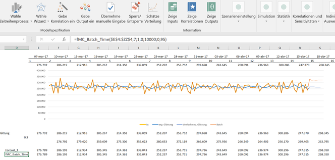
In MC FLO, a number is calculated using a random experiment. This number changes as the experiment is repeated. This distinguishes the (stochastic) time series processes from deterministic approaches such as the already mentioned exponential smoothing. A large number of random experiments (here 10'000) should be chosen so that the quality of the prognosis can be considered sufficient. With the quantile barrier (or percentile, here 95%) you control the target size based on risk. After the batch run, we see that MC FLO has selected an MA process (recognizable by the comment in cell D25 inserted by MC FLO, and thus according to our consideration above), and an occupancy of just under 322k for the 95% quantile for the seventh week. As we said, this value has a "probability" of 5% that the effective occupancy number can be higher than the predicted one. Finally, it can be seen that the predicted numbers are in line with the realized occupancy and therefore the reasoning of an MA process seems justified.

The big "wow" of the batch function resides in the high level of automation through supported machine learning and transparency. Once you have entered the data for the following week, all you need to do is start a new forecast under «Other», «Start Batch», which will automatically generate a suitable process in a first step and then update all formulas starting with «= fMC_Batch_Time». So you can easily install a rolling planning / forecasting into your Excel models in real time. Try it!
Kommentar schreiben