The moving average model - behind the scenes

In one of our last blogs (in german) we have deepened the AR (auto-regressive) time series model and presented a practical example in relation to the method of moments implemented in MC FLO. At this point we would like to do the same for the MA (moving-average) time series process.

An MA process of first order consists primarily of a recurring constant value - the expected value - and a random component at each period, which correlates over the course of time and superimposes the expected value. The special feature of an MA process is therefore the unobservable and correlated random values. Here's an example: Imagine you sell coffee capsules and the average sales is 200,000. In addition to the direct sale, you also offer coupon stamps (with expiration date), which should promote sales and which are promoted by third parties. Each coupon promotion can be individually designed by the third party and coupled with other products. Thus, you cannot directly control and monitor the market for vouchers for your capsules. In the case of an MA(1) model, therefore, the sales in the current period will be based on the number of coupon campaigns in that period and with a weighting on the coupon campaign of the last period (that is, coupons issued in the last period will be redeemed in the this period).

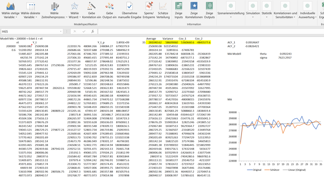
In the following Excel we have prepared the logic of MC FLO in relation to the MA(1) model. In column B we have depicted 35 normal random numbers with a mean of 50,000 and a standard deviation of 5,000. The MA process should be designed such that the expected value is 200,000 and the random number of the previous period is included with a weight of 0.6. With this we have reproduced the above described coffee example. Column C picks up these random numbers and uses the formula entered in cell A1 to map the corresponding MA(1) process. For the theta - the weight of the previous period - a value of 0.09 is shown by the method of moments and an amount of 7'623 for the standard deviation. The determination of the parameters using MC FLO supplies the same numbers. Compared to the real parameters of 0.6 and 5'000 this reflect a relatively high deviation. To validate the method of moments, we can use the better estimation method "maximum likelihood". For this we used the open source tool "gretl". In this case the theta is 0.48 and a standard deviation of 7'767 is determined.At least in terms of the weighting (theta), the maximum likelihood is superior to the method of moments. 

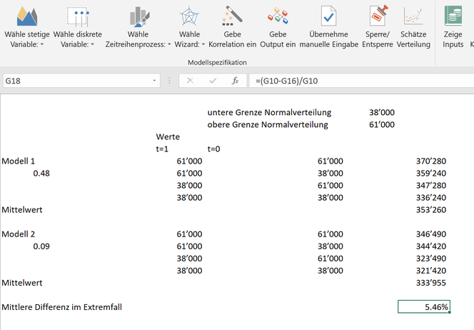
The fact that both methods estimate the model parameters relatively poorly is due to the small size of the test data (35 observations) and the specification of the random term. Compared to the maximum likelihood, however, it is not the deviation of the parameters that is of primary relevance, but the ability to make an appropriate estimate based on the chosen model and parameters. For the 95% confidence interval (meaning that in 1'000 repetitions of the random experiment a score would be within the confidence interval in 950 cases), for the fifth forecast day (day 40) "gretl" calculates a lower bound of 264,424 and an upper bound of 296,819. Using 10,000 iterations and with the batch function of MC FLO, we come to values of 266,512 and 295,970. These values are quite similar and yet at first glance amazing, because at a theta of 0.48 the previous period is obviously weighted more heavily than at a value of 0.09. This should lead to a much higher deviation, right? If we limit the normally distributed random variable (mean of 50,000 and standard deviation of 5,000) in practice to the 98% confidence interval, we get 38,000 as the lower limit and 61,000 as the upper limit. Below we have outlined the four possible extreme constellations and the implications for an MA(1) process. The average difference is just 5% using the minimum and the maximum, based on a calculated expected mean of rounded 280,000 in both models (the details can be found in the formulas). It is obvious that not only the theta should be used as a measure for a good model. From this practical consideration we are convinced that the method of moments is sufficient for the MA(1) model.

As a rule, phenomena such as the coupon campaigns are not independent of other variables which, for example, influence the profit of a company. For each voucher campaign, an amount will be paid to the issuer. The higher the complexity of the voucher campaigns, the higher the costs for the company concerned. Here, in contrast to the AR process, however, not the entire sales of coffee capsules, but only the effort triggered by coupon campaigns are relevant. Therefore, the random numbers per period are to be correlated with the corresponding costs, here simplified with a PERT distribution. In addition, we would like to assume that the payments to the issues are only dependent on the campaigns.

Consequently, only the coffee capsule manufacturer profits from vouchers redeemed later. Since there is an almost perfect correlation and the cause-relationship is also clear, we have used a correlation coefficient of 0.999 (technically no relation of exactly 1 can be taken in MC FLO, therefore smaller values are to be used, but this does not imply any practical  restriction). Thus, we can model the impact of a coupon campaign on our profit directly as a risk-based simulation in MC FLO. It makes sense, of course, that the weighting of the previous period as part of the MA process is also modeled, since we should take into account as fully as possible the uncertain occurrences (here the redemption rate from the previous period) in our simulation.

Analogously we have set here a PERT distribution with a modal value of 0.6. After 10,000 iterations, taking the correlation into account, we arrive at a surcharge profit of 47 TCHF on average (we have set each sale at 1 CHF and neglected other variables, such as own distribution costs, etc.). More importantly, however, is the observation that the costs of the coupon campaigns in most of the iterations studied are lower than the extra yield. Say, only with a 30% certainty a coupon campaign for the coffee capsule manufacturer is more expensive than the expected surplus. 

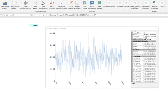
In MC FLO, you can use the MA(1) process as an integral part of a simulation with only one variable. Therefore, you do not have to define the variables defined in the coffee capsule model individually. An integrated simulation is particularly useful if you have to make predictions for the future and you have obtained an MA(1) process as a starting position based on the estimation function of MC FLO.

We have to admit that the economics of coupons is much more complicated than the simplification presented here.