
Our intention in the following blog post is to embrace corporate planning with modern generative models (Bayesian statistics) and define terms such as “ambition” and “prediction” in a refreshingly new way. You will be amazed that this kind of planning process, which combines subjective assessments with data, can be set up with Excel and MC FLO without large investments in planning suites.
For companies, planning means - in simplified terms - unmantling the processes that are required to create the services / products offered on the market - from sales flow to costs - with the aim to identify the key drivers that are relevant for performance and to shape them in such a way that the company value is maximized.
It should be noted that future outcome is uncertain and the figures to be taken into account during the planning process will be subject to fluctuations around an initial plan value. A company that has to dimension production capacities, for example, cannot rely solely on mean or expected values. It has to assess the full range of all possible outcomes with their corresponding probabilities to make the right decisions. In addition, deviations from target values (= ambition) must be identified and new knowledge based on the data must be taken into account to derive predictions.
To solve all of these problems, Bayesian statistics in combination with the Monte Carlo approach provides the necessary framework to make the planning process reliable.
To avoid all mathematical formulas, we start from the following situation: A newly founded company wants to provide repair services for watches in region A. As a sub-task, the management has to set up the sales planning for the first year. Since no data are available for the company so far, estimates have to be used.
Let us assume that, based on previous experience in the watch industry, management has made the following assumptions for one year (= 240 working days), which can be described by a triangular distribution.
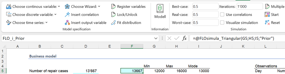
The management assumes that a minimum of 12,000 chargeable repair orders will be carried out within one year, a maximum of 16,000 and a most probable value of 13,000. This “estimate” can be represented as a probability distribution and, in the sense of Bayesian statistics, represents our prior knowledge (“beliefs”, “a priori”).
The initial set-up of the planning process requires - in the absence of data - assumptions, which are quantified.
In relation to the number of repair orders, following conclusions can be derived on the basis of a simulation:
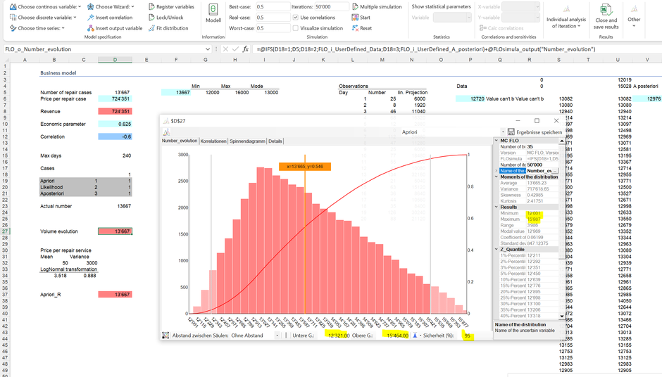
A minimum of 12,001 and a maximum of 15,987 repair orders are calculated for the year, so the values do not deviate significantly from the theoretical minimum and maximum. 95% of the results are between 12,321 and 15,464. The fluctuations between the minimum and the maximum represent the uncertainty. Low values can be seen as part of worst-case scenarios, whereby high demand is more probable in best-case scenarios.
The same procedure as described above can be used to derive the transfer prices. A simple battery change is priced differently than a revision of a watch with a tourbillon. We assume that the price flow can be approximated by a log-normal distribution, i.e. also analytically (see column B30ff). However, nothing prevents management from entering a user-defined function via a histogram (which can't be tracked analytically, only numerically). This is the core of Bayesian statistics: There is no such thing as “true” or “false”, rather “well founded” and “less well founded”. “Less good” assumptions can be adjusted based on the data available (more on this later)*.
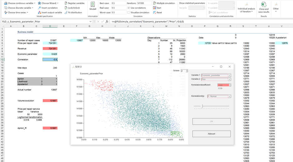
A robust planning approach covers all relevant drivers. Or to put it another way: A model and thus the informative value of a plan depends on the assumptions. Let us finally assume that the number of repair orders depends on the expectation of the economic situation: If the economy is growing, consumers are more likely to buy new watches rather than to repair existing ones and vice versa. This dependency can be viewed numerically as a correlation and is shown in cell D12.
As the relevant performance indicator, the management is interested in the revenue stream for the next year. Using the convolution concept, the product of both variables (quantity, price) yields the revenue distribution from which predictions - using our prior beliefs - can be derived:
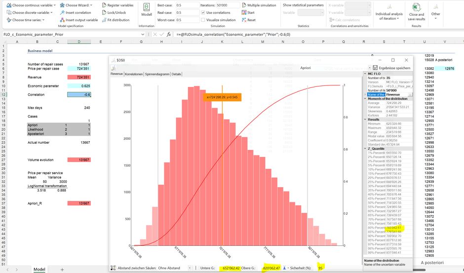
So we see that 95% of the results are between 0.65 MCHF and 0.82 MCHF. Analogously as above, we can make the following statement: "Based on our beliefs, we can be 95% certain that the revenue within one year will be between 0.65 MCHF and 0.82 CHF". From such statement, the “ambition” can be derived. If the management sets a revenue target of 0.5 MCHF, the probability of exceeding this target would be 100% and therefore not ambitious (the simulated minimum of approx. 0.62 MCHF is above this sales target). On the other hand, a revenue target of 1 MCHF would be ambitious, but not achievable.
An ambition of 20% (or in other words: 80% of the results are below this value) is equivalent to a sales target of at least CHF 766,000. This goal can be achieved, but only with a probability of 20%. It is key task of the management to define the specific ambition level in advance or when data is available.
Let us assume that the management has set an ambition of 30% and thus expects a sales target of approx. 748,000 CHF.
The planning process, which defines the interaction of the relevant drivers and closes with the goal setting, is thus completed in our case (reality is naturally more complex [behaviour of competitors etc.]). If new drivers, for example due to an expanded business model, or previous drivers are to be replaced by others, the model must be adapted. This model update process has to be separated from the question of when and how to update the parameters in order to measure the achievement of our objectives.
After one month (= 20 working days), the first data on the billable repair orders are available:
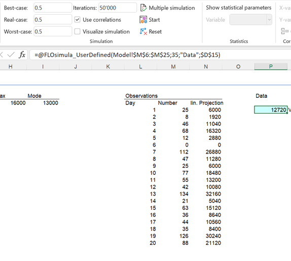
No repair orders were carried out on day 6; however, the highest measured number of repair orders within a day is 134 (day 13). Bayesian statistics allow us to combine the data (“evidence”) with our previous knowledge in order to derive an updated knowledge (posteriori). To do this, the first thing to do is to determine the likelihood function from the data. That sounds very technical, but is relatively easy to implement for most planning tasks. The idea is this: Given that we only had this data and we had to make a prediction for a year, how would we proceed? We are therefore looking for combinations that maximize the likely observable values. This is then our likelihood. A common approach is to use "bootstrap": we pick randomly from the observed data 240 times a number of repair orders and add them up. Here the resulting distribution
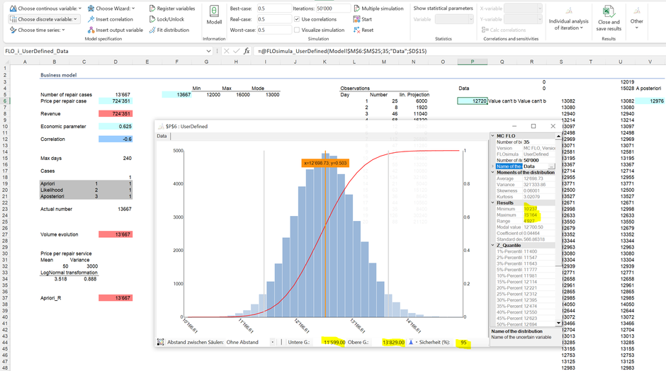
The likelihood function shows that the expected repair orders based on the data are likely to fluctuate between 10,237 and 15,164 in a year. In combination with the price function, this results in the following likelihood for the revenue (for the sake of simplicity, we assume that the evidence on prices and the correlation is equal our prior knowledge):
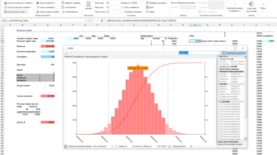
With regard to the likelihood, 95% of the results are between 0.61 MCHF and 0.73 MCHF; the maximum at just 0.81 MCHF.
The next step is to combine the revenue likelihood function with our prior knowledge. With the corresponding MC FLO formula "fMC_BayesMCMC", a sample is made from the so-called posteriori distribution. Like the prior knowledge, this posterior distribution can also be used to asserts predictions**.

In 95% of the cases the turnover will be between 0.65 and 0.73 MCHF after one year. In contrast, the probability that sales will exceed the target of 0.77 MCHF is now less than 1%.
Management uses the observed data and the resulting posteriori distribution to decide whether it would like to maintain the previously defined ambition or whether it should adjust it's assumptions based on the data (it can even adjusts it's prior knowledge [the likelihood's minimum is not supported by the prior]). Management can wait another month and then use the new data to combine it with the “prior knowledge” (our calculated posteriori distribution) to obtain an updated posteriori distribution. However, if the original ambition is retained, it can define the measures that contribute to an increase in expected sales. Since it cannot actually influence the external factors - such as the assessment of the economic situation - our model setting only permits the opportunity to adjusts the prices.
Conclusion: Bayesian statistics in conjunction with the Monte Carlo approach can be used effectively for corporate planning. It is based on the concept of prior knowledge (a priori), which quantifies subjective assessments and allows this prior knowledge to be updated on the basis of new data. By quantifying all possible future outcomes (scenarios), ambitions (target values) can be consistently derived and predictions performed.
* Risk studies shows that people are exposed to biases in the compilation of prior knowledge (e.g. by incorrectly assessing probabilities). This is true, but as far we use data to update our knowledge, these biases are thinned in the course of time.
** Many people think that we should only rely on the data - in this case the likelihood. But this is clearly to be denied from a Bayesian view. What if the data at hand does not yet reflect the whole truth? This is exactly why our prior knowledge is important. In the course of time, the data will - if the prior knowledge was not classified as «absolute» - dominate.
Anecdote: The modern statistics developed by reverent Thomas Bayes independently of Laplace only became public after his death. One suspicion is that Bayes rejected a publication because the transition from prior beliefs using data to the adapted knowledge (posterior) contradicts the unconditional belief in God. The famous Bayesian formula makes only sense if the prior knowledge is not declared as absolute, otherwise even the best data cannot lead to an adapted knowledge. In other words: Doubts about the existence of God are necessary so that the previous knowledge can be converted into an adapted posteriori knowledge, given the data.
Here is a comparison of the various distributions concerning the revenue stream.

The graphic helps to explain the determination of the posteriori distribution using the Metropolis-Hasting algorithm: For values that are contained both in our prior and in the likelihood, there is a high probability that these will be included in the posteriori distribution; on the other hand, the probability of admission decreases if the values differ and are far apart (as we can see, some values of the likelihood are not contained in the posterior distribution. This is due that our prior distribution has a left threshold [12,000], imposing thus a limitation on the posterior distribution. It follows that the prior belief should contain all feasible outcomes [revenue of zero]!).
The functions presented and the corresponding Excel-workbook are available from MC FLO version 7.6 and above.
This blog post has been used with German localization enabled on Microsoft Excel.
Kommentar schreiben